Using ReX interactively
There are three key components that need to be set up in order to use ReX: the input parameters, the model, and the input data. In this tutorial we will walk through how to set up each of these for a simple ReX analysis using an image classification model. We will use ReX to calculate a responsibility landscape and identify a minimal explanation for the classification of an image by the ResNet50 model. We will also plot this explanation and the responsibility landscape on the original image.
Set up
First, we will set up the input parameters as a CausalArgs object.
You can create a CausalArgs object with default parameters and then modify it, or use load_config to read your desired set of input parameters from a rex.toml file.
from rex_xai.config import CausalArgs

args = CausalArgs()
print(args)
Causal Args <Args <file: , model: None, gpu: True, mode: None, progress_bar: True, output_file: None, surface_plot: None, heatmap_plot: None, onnx_means: None, onnx_stds: None, onnx_norm: 255.0 onnx_inter_op_threads: 8, onnx_intra_op_threads: 8, onnx_logger: 3explanation_strategy: Strategy.Global, min_confidence_scalar: 0.0, chunk size: 10, spatial_radius: 25, spatial_eta: 0.2, seed: None, db: None, script: None, verbosity: 1, spotlights: 10, spotlight_size: 20, spotlight_eta: 0.2, no_expansions: 4, obj_function: none, config_location: None, mask_value: 0, tree_depth: 10, search_limit: None, min_box_size: 10, weighted: False, confidence_filter: 0.0, data_locations: None, distribution: Distribution.Uniform, distribution_args: None, queue_len: 1, queue_style Queue.Area, concentrate: False, iterations: 20>
For the purpose of this tutorial we will set gpu = False and use 10 iterations. We will also set a seed to ensure reproducible outputs.
args.gpu = False
args.iters = 10
args.seed = 123
print(args)
Causal Args <Args <file: , model: None, gpu: False, mode: None, progress_bar: True, output_file: None, surface_plot: None, heatmap_plot: None, onnx_means: None, onnx_stds: None, onnx_norm: 255.0 onnx_inter_op_threads: 8, onnx_intra_op_threads: 8, onnx_logger: 3explanation_strategy: Strategy.Global, min_confidence_scalar: 0.0, chunk size: 10, spatial_radius: 25, spatial_eta: 0.2, seed: 123, db: None, script: None, verbosity: 1, spotlights: 10, spotlight_size: 20, spotlight_eta: 0.2, no_expansions: 4, obj_function: none, config_location: None, mask_value: 0, tree_depth: 10, search_limit: None, min_box_size: 10, weighted: False, confidence_filter: 0.0, data_locations: None, distribution: Distribution.Uniform, distribution_args: None, queue_len: 1, queue_style Queue.Area, concentrate: False, iterations: 10>
Next, we will set up the model details. We need to provide ReX with three things:
the shape the model expects the input data to be
a preprocessing function that will apply the appropriate transforms to the input data
a prediction function to be applied to the transformed input data
For this tutorial we will use the ResNet50 model as provided by the torchvision library.
from torchvision.models import resnet50

model = resnet50(weights="ResNet50_Weights.DEFAULT")
model.eval()
model.to("cpu")
Show code cell output
Downloading: "https://download.pytorch.org/models/resnet50-11ad3fa6.pth" to /home/docs/.cache/torch/hub/checkpoints/resnet50-11ad3fa6.pth
0%| | 0.00/97.8M [00:00<?, ?B/s]
39%|███▉ | 38.0M/97.8M [00:00<00:00, 398MB/s]
78%|███████▊ | 76.0M/97.8M [00:00<00:00, 385MB/s]
100%|██████████| 97.8M/97.8M [00:00<00:00, 392MB/s]
ResNet(
  (conv1): Conv2d(3, 64, kernel_size=(7, 7), stride=(2, 2), padding=(3, 3), bias=False)
  (bn1): BatchNorm2d(64, eps=1e-05, momentum=0.1, affine=True, track_running_stats=True)
  (relu): ReLU(inplace=True)
  (maxpool): MaxPool2d(kernel_size=3, stride=2, padding=1, dilation=1, ceil_mode=False)
  (layer1): Sequential(
    (0): Bottleneck(
      (conv1): Conv2d(64, 64, kernel_size=(1, 1), stride=(1, 1), bias=False)
      (bn1): BatchNorm2d(64, eps=1e-05, momentum=0.1, affine=True, track_running_stats=True)
      (conv2): Conv2d(64, 64, kernel_size=(3, 3), stride=(1, 1), padding=(1, 1), bias=False)
      (bn2): BatchNorm2d(64, eps=1e-05, momentum=0.1, affine=True, track_running_stats=True)
      (conv3): Conv2d(64, 256, kernel_size=(1, 1), stride=(1, 1), bias=False)
      (bn3): BatchNorm2d(256, eps=1e-05, momentum=0.1, affine=True, track_running_stats=True)
      (relu): ReLU(inplace=True)
      (downsample): Sequential(
        (0): Conv2d(64, 256, kernel_size=(1, 1), stride=(1, 1), bias=False)
        (1): BatchNorm2d(256, eps=1e-05, momentum=0.1, affine=True, track_running_stats=True)
      )
    )
    (1): Bottleneck(
      (conv1): Conv2d(256, 64, kernel_size=(1, 1), stride=(1, 1), bias=False)
      (bn1): BatchNorm2d(64, eps=1e-05, momentum=0.1, affine=True, track_running_stats=True)
      (conv2): Conv2d(64, 64, kernel_size=(3, 3), stride=(1, 1), padding=(1, 1), bias=False)
      (bn2): BatchNorm2d(64, eps=1e-05, momentum=0.1, affine=True, track_running_stats=True)
      (conv3): Conv2d(64, 256, kernel_size=(1, 1), stride=(1, 1), bias=False)
      (bn3): BatchNorm2d(256, eps=1e-05, momentum=0.1, affine=True, track_running_stats=True)
      (relu): ReLU(inplace=True)
    )
    (2): Bottleneck(
      (conv1): Conv2d(256, 64, kernel_size=(1, 1), stride=(1, 1), bias=False)
      (bn1): BatchNorm2d(64, eps=1e-05, momentum=0.1, affine=True, track_running_stats=True)
      (conv2): Conv2d(64, 64, kernel_size=(3, 3), stride=(1, 1), padding=(1, 1), bias=False)
      (bn2): BatchNorm2d(64, eps=1e-05, momentum=0.1, affine=True, track_running_stats=True)
      (conv3): Conv2d(64, 256, kernel_size=(1, 1), stride=(1, 1), bias=False)
      (bn3): BatchNorm2d(256, eps=1e-05, momentum=0.1, affine=True, track_running_stats=True)
      (relu): ReLU(inplace=True)
    )
  )
  (layer2): Sequential(
    (0): Bottleneck(
      (conv1): Conv2d(256, 128, kernel_size=(1, 1), stride=(1, 1), bias=False)
      (bn1): BatchNorm2d(128, eps=1e-05, momentum=0.1, affine=True, track_running_stats=True)
      (conv2): Conv2d(128, 128, kernel_size=(3, 3), stride=(2, 2), padding=(1, 1), bias=False)
      (bn2): BatchNorm2d(128, eps=1e-05, momentum=0.1, affine=True, track_running_stats=True)
      (conv3): Conv2d(128, 512, kernel_size=(1, 1), stride=(1, 1), bias=False)
      (bn3): BatchNorm2d(512, eps=1e-05, momentum=0.1, affine=True, track_running_stats=True)
      (relu): ReLU(inplace=True)
      (downsample): Sequential(
        (0): Conv2d(256, 512, kernel_size=(1, 1), stride=(2, 2), bias=False)
        (1): BatchNorm2d(512, eps=1e-05, momentum=0.1, affine=True, track_running_stats=True)
      )
    )
    (1): Bottleneck(
      (conv1): Conv2d(512, 128, kernel_size=(1, 1), stride=(1, 1), bias=False)
      (bn1): BatchNorm2d(128, eps=1e-05, momentum=0.1, affine=True, track_running_stats=True)
      (conv2): Conv2d(128, 128, kernel_size=(3, 3), stride=(1, 1), padding=(1, 1), bias=False)
      (bn2): BatchNorm2d(128, eps=1e-05, momentum=0.1, affine=True, track_running_stats=True)
      (conv3): Conv2d(128, 512, kernel_size=(1, 1), stride=(1, 1), bias=False)
      (bn3): BatchNorm2d(512, eps=1e-05, momentum=0.1, affine=True, track_running_stats=True)
      (relu): ReLU(inplace=True)
    )
    (2): Bottleneck(
      (conv1): Conv2d(512, 128, kernel_size=(1, 1), stride=(1, 1), bias=False)
      (bn1): BatchNorm2d(128, eps=1e-05, momentum=0.1, affine=True, track_running_stats=True)
      (conv2): Conv2d(128, 128, kernel_size=(3, 3), stride=(1, 1), padding=(1, 1), bias=False)
      (bn2): BatchNorm2d(128, eps=1e-05, momentum=0.1, affine=True, track_running_stats=True)
      (conv3): Conv2d(128, 512, kernel_size=(1, 1), stride=(1, 1), bias=False)
      (bn3): BatchNorm2d(512, eps=1e-05, momentum=0.1, affine=True, track_running_stats=True)
      (relu): ReLU(inplace=True)
    )
    (3): Bottleneck(
      (conv1): Conv2d(512, 128, kernel_size=(1, 1), stride=(1, 1), bias=False)
      (bn1): BatchNorm2d(128, eps=1e-05, momentum=0.1, affine=True, track_running_stats=True)
      (conv2): Conv2d(128, 128, kernel_size=(3, 3), stride=(1, 1), padding=(1, 1), bias=False)
      (bn2): BatchNorm2d(128, eps=1e-05, momentum=0.1, affine=True, track_running_stats=True)
      (conv3): Conv2d(128, 512, kernel_size=(1, 1), stride=(1, 1), bias=False)
      (bn3): BatchNorm2d(512, eps=1e-05, momentum=0.1, affine=True, track_running_stats=True)
      (relu): ReLU(inplace=True)
    )
  )
  (layer3): Sequential(
    (0): Bottleneck(
      (conv1): Conv2d(512, 256, kernel_size=(1, 1), stride=(1, 1), bias=False)
      (bn1): BatchNorm2d(256, eps=1e-05, momentum=0.1, affine=True, track_running_stats=True)
      (conv2): Conv2d(256, 256, kernel_size=(3, 3), stride=(2, 2), padding=(1, 1), bias=False)
      (bn2): BatchNorm2d(256, eps=1e-05, momentum=0.1, affine=True, track_running_stats=True)
      (conv3): Conv2d(256, 1024, kernel_size=(1, 1), stride=(1, 1), bias=False)
      (bn3): BatchNorm2d(1024, eps=1e-05, momentum=0.1, affine=True, track_running_stats=True)
      (relu): ReLU(inplace=True)
      (downsample): Sequential(
        (0): Conv2d(512, 1024, kernel_size=(1, 1), stride=(2, 2), bias=False)
        (1): BatchNorm2d(1024, eps=1e-05, momentum=0.1, affine=True, track_running_stats=True)
      )
    )
    (1): Bottleneck(
      (conv1): Conv2d(1024, 256, kernel_size=(1, 1), stride=(1, 1), bias=False)
      (bn1): BatchNorm2d(256, eps=1e-05, momentum=0.1, affine=True, track_running_stats=True)
      (conv2): Conv2d(256, 256, kernel_size=(3, 3), stride=(1, 1), padding=(1, 1), bias=False)
      (bn2): BatchNorm2d(256, eps=1e-05, momentum=0.1, affine=True, track_running_stats=True)
      (conv3): Conv2d(256, 1024, kernel_size=(1, 1), stride=(1, 1), bias=False)
      (bn3): BatchNorm2d(1024, eps=1e-05, momentum=0.1, affine=True, track_running_stats=True)
      (relu): ReLU(inplace=True)
    )
    (2): Bottleneck(
      (conv1): Conv2d(1024, 256, kernel_size=(1, 1), stride=(1, 1), bias=False)
      (bn1): BatchNorm2d(256, eps=1e-05, momentum=0.1, affine=True, track_running_stats=True)
      (conv2): Conv2d(256, 256, kernel_size=(3, 3), stride=(1, 1), padding=(1, 1), bias=False)
      (bn2): BatchNorm2d(256, eps=1e-05, momentum=0.1, affine=True, track_running_stats=True)
      (conv3): Conv2d(256, 1024, kernel_size=(1, 1), stride=(1, 1), bias=False)
      (bn3): BatchNorm2d(1024, eps=1e-05, momentum=0.1, affine=True, track_running_stats=True)
      (relu): ReLU(inplace=True)
    )
    (3): Bottleneck(
      (conv1): Conv2d(1024, 256, kernel_size=(1, 1), stride=(1, 1), bias=False)
      (bn1): BatchNorm2d(256, eps=1e-05, momentum=0.1, affine=True, track_running_stats=True)
      (conv2): Conv2d(256, 256, kernel_size=(3, 3), stride=(1, 1), padding=(1, 1), bias=False)
      (bn2): BatchNorm2d(256, eps=1e-05, momentum=0.1, affine=True, track_running_stats=True)
      (conv3): Conv2d(256, 1024, kernel_size=(1, 1), stride=(1, 1), bias=False)
      (bn3): BatchNorm2d(1024, eps=1e-05, momentum=0.1, affine=True, track_running_stats=True)
      (relu): ReLU(inplace=True)
    )
    (4): Bottleneck(
      (conv1): Conv2d(1024, 256, kernel_size=(1, 1), stride=(1, 1), bias=False)
      (bn1): BatchNorm2d(256, eps=1e-05, momentum=0.1, affine=True, track_running_stats=True)
      (conv2): Conv2d(256, 256, kernel_size=(3, 3), stride=(1, 1), padding=(1, 1), bias=False)
      (bn2): BatchNorm2d(256, eps=1e-05, momentum=0.1, affine=True, track_running_stats=True)
      (conv3): Conv2d(256, 1024, kernel_size=(1, 1), stride=(1, 1), bias=False)
      (bn3): BatchNorm2d(1024, eps=1e-05, momentum=0.1, affine=True, track_running_stats=True)
      (relu): ReLU(inplace=True)
    )
    (5): Bottleneck(
      (conv1): Conv2d(1024, 256, kernel_size=(1, 1), stride=(1, 1), bias=False)
      (bn1): BatchNorm2d(256, eps=1e-05, momentum=0.1, affine=True, track_running_stats=True)
      (conv2): Conv2d(256, 256, kernel_size=(3, 3), stride=(1, 1), padding=(1, 1), bias=False)
      (bn2): BatchNorm2d(256, eps=1e-05, momentum=0.1, affine=True, track_running_stats=True)
      (conv3): Conv2d(256, 1024, kernel_size=(1, 1), stride=(1, 1), bias=False)
      (bn3): BatchNorm2d(1024, eps=1e-05, momentum=0.1, affine=True, track_running_stats=True)
      (relu): ReLU(inplace=True)
    )
  )
  (layer4): Sequential(
    (0): Bottleneck(
      (conv1): Conv2d(1024, 512, kernel_size=(1, 1), stride=(1, 1), bias=False)
      (bn1): BatchNorm2d(512, eps=1e-05, momentum=0.1, affine=True, track_running_stats=True)
      (conv2): Conv2d(512, 512, kernel_size=(3, 3), stride=(2, 2), padding=(1, 1), bias=False)
      (bn2): BatchNorm2d(512, eps=1e-05, momentum=0.1, affine=True, track_running_stats=True)
      (conv3): Conv2d(512, 2048, kernel_size=(1, 1), stride=(1, 1), bias=False)
      (bn3): BatchNorm2d(2048, eps=1e-05, momentum=0.1, affine=True, track_running_stats=True)
      (relu): ReLU(inplace=True)
      (downsample): Sequential(
        (0): Conv2d(1024, 2048, kernel_size=(1, 1), stride=(2, 2), bias=False)
        (1): BatchNorm2d(2048, eps=1e-05, momentum=0.1, affine=True, track_running_stats=True)
      )
    )
    (1): Bottleneck(
      (conv1): Conv2d(2048, 512, kernel_size=(1, 1), stride=(1, 1), bias=False)
      (bn1): BatchNorm2d(512, eps=1e-05, momentum=0.1, affine=True, track_running_stats=True)
      (conv2): Conv2d(512, 512, kernel_size=(3, 3), stride=(1, 1), padding=(1, 1), bias=False)
      (bn2): BatchNorm2d(512, eps=1e-05, momentum=0.1, affine=True, track_running_stats=True)
      (conv3): Conv2d(512, 2048, kernel_size=(1, 1), stride=(1, 1), bias=False)
      (bn3): BatchNorm2d(2048, eps=1e-05, momentum=0.1, affine=True, track_running_stats=True)
      (relu): ReLU(inplace=True)
    )
    (2): Bottleneck(
      (conv1): Conv2d(2048, 512, kernel_size=(1, 1), stride=(1, 1), bias=False)
      (bn1): BatchNorm2d(512, eps=1e-05, momentum=0.1, affine=True, track_running_stats=True)
      (conv2): Conv2d(512, 512, kernel_size=(3, 3), stride=(1, 1), padding=(1, 1), bias=False)
      (bn2): BatchNorm2d(512, eps=1e-05, momentum=0.1, affine=True, track_running_stats=True)
      (conv3): Conv2d(512, 2048, kernel_size=(1, 1), stride=(1, 1), bias=False)
      (bn3): BatchNorm2d(2048, eps=1e-05, momentum=0.1, affine=True, track_running_stats=True)
      (relu): ReLU(inplace=True)
    )
  )
  (avgpool): AdaptiveAvgPool2d(output_size=(1, 1))
  (fc): Linear(in_features=2048, out_features=1000, bias=True)
)
We need to define a model_shape object which is a list with the expected shape of the input data for the model. In this case the order is [batch, channels, height, width]. We use “N” for the batch size in this case as this model accepts dynamic batch sizes. The actual batch size used can be set in the CausalArgs object.
model_shape = ["N", 3, 224, 224]
We also need to define a preprocess function which will be applied to our input data file, and return a ReX Data object that has been appropriately transformed.
The transformations (e.g. resizing, normalisation) should be the same as were used for the model’s training. For this model, we use the following transformations:
from torchvision import transforms as T
from PIL import Image

from rex_xai.input_data import Data

def preprocess(path, shape, device, mode) -> Data:
    transform = T.Compose(
        [
            T.Resize((224, 224)),
            T.ToTensor(),
            T.Normalize(mean=[0.485, 0.456, 0.406], std=[0.229, 0.224, 0.225]),
        ]
    )
    img = Image.open(path).convert("RGB")
    data = Data(img, shape, device, mode=mode, process=False)
    data.data = transform(img).unsqueeze(0).to(device)
    data.mode = "RGB"
    data.model_shape = shape
    data.model_height = 224
    data.model_width = 224
    data.model_channels = 3
    data.transposed = True
    data.model_order = "first"

    return data
Finally, we will define a prediction_function that will be applied to our input data and mutants:
import torch as tt
import torch.nn.functional as F

from rex_xai.prediction import from_pytorch_tensor

def prediction_function(mutants, target=None, raw=False, binary_threshold=None):
    with tt.no_grad():
        tensor = model(mutants)
        if raw:
            return F.softmax(tensor, dim=1)
        return from_pytorch_tensor(tensor)
Now we are almost ready to run ReX. The final step is to set up the input data.
from rex_xai.explanation import load_and_preprocess_data, predict_target
from rex_xai._utils import get_device
device = get_device(gpu=False)
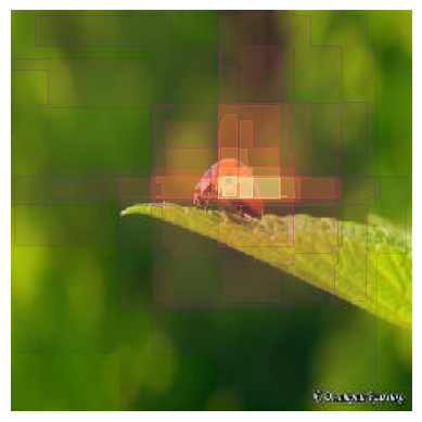
args.path = '../../tests/test_data/ladybird.jpg'
data = load_and_preprocess_data(model_shape, device, args)
This is our input image:
Image.open(args.path)

We will now set the mask value to be used to mask the data when creating mutants, and predict the class of the original input image (the ‘target’ for the mutants).
ReX allows functions to be used to set the mask value (e.g. the ‘min’ or ‘mean’ of the normalised image), but the default mask value of 0 generally performs well enough for images.
data.set_mask_value(0)
data.target = predict_target(data, prediction_function)
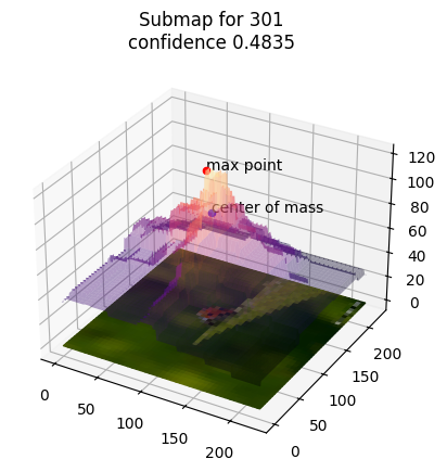
print(data.target)
FOUND_CLASS: 301, FOUND_CONF: 0.48350, TARGET_CLASS: n/a, TARGET_CONFIDENCE: n/a
Running ReX
We are now ready to run ReX and identify a causal explanation for this classification.
The main function in ReX is calculate_responsibility, which returns a ResponsibilityMaps object and some statistics about the function execution.
We can then create an Explanation object containing the calculated responsibility landscape and extract an explanation from this object.
Here we will use the Global strategy. Additional strategies are available in the rex_xai._utils.Strategy Enum.
from rex_xai.explanation import calculate_responsibility
from rex_xai.extraction import Explanation
from rex_xai._utils import Strategy

resp_maps, stats = calculate_responsibility(data, args, prediction_function)
exp = Explanation(resp_maps, prediction_function, data, args, stats)
exp.extract(Strategy.Global)
Show code cell output
0%| | 0/10 [00:00<?, ?it/s]
10%|█ | 1/10 [00:08<01:13, 8.22s/it]
20%|██ | 2/10 [00:18<01:17, 9.72s/it]
30%|███ | 3/10 [00:27<01:02, 8.95s/it]
40%|████ | 4/10 [00:39<01:01, 10.21s/it]
50%|█████ | 5/10 [00:51<00:54, 10.93s/it]
60%|██████ | 6/10 [00:59<00:40, 10.03s/it]
70%|███████ | 7/10 [01:14<00:35, 11.70s/it]
80%|████████ | 8/10 [01:24<00:22, 11.06s/it]
90%|█████████ | 9/10 [01:34<00:10, 10.61s/it]
100%|██████████| 10/10 [01:47<00:00, 11.47s/it]
100%|██████████| 10/10 [01:47<00:00, 10.75s/it]
Examining the results
The mask corresponding to the final explanation is stored in the Explanation object and can be printed:
print(exp.final_mask)
[[[False False False ... False False False]
  [False False False ... False False False]
  [False False False ... False False False]
  ...
  [False False False ... False False False]
  [False False False ... False False False]
  [False False False ... False False False]]

 [[False False False ... False False False]
  [False False False ... False False False]
  [False False False ... False False False]
  ...
  [False False False ... False False False]
  [False False False ... False False False]
  [False False False ... False False False]]

 [[False False False ... False False False]
  [False False False ... False False False]
  [False False False ... False False False]
  ...
  [False False False ... False False False]
  [False False False ... False False False]
  [False False False ... False False False]]]
ReX also provides some plotting methods for easier visualisation of the explanation and the responsibility landscape.
display(exp.show())

The responsibility landscape can be plotted as a heatmap or 3D surface plot:
exp.heatmap_plot()
exp.surface_plot()
If you are not satisfied with the quality of the explanation output, a good place to start is to check the run statistics output by calculate_responsibility.
In particular, check the tree depth and numbers of mutants examined, as low tree depth or low numbers of mutants examined can lead to strange results. The easiest way to increase both of these and refine an explanation is to increase the number of iterations you use.
print(stats)
{'total_passing': 343, 'total_failing': 763, 'max_depth_reached': 7, 'avg_box_size': 373.00416666666666}
In this case, the tree depth is 9, almost 1000 mutants have been assessed, and the returned explanation matches well with what we would expect, so we are happy with the quality of the explanation and don’t need to increase the iterations.
Another way to check explanation quality would be to analyze the Explanation object and calculate some common metrics.
from rex_xai.explanation import analyze

analyze(exp, data.mode)
{'area': 0.0027901785714285715,
 'entropy': 6.632282108140689,
 'max_entropy': None,
 'insertion_curve': 0.8735558874984664,
 'deletion_curve': 0.04179783858644}
Multiple Explanations
There may be multiple regions of an image that are sufficient to explain its classification.
ReX provides a way to identify multiple explanations by using the MultiExplanation class and MultiSpotlight strategy.
We will use a different image to illustrate this approach, so we need to set up the Data object for this new image.
We will copy the args object and change the path to point to the new data.
import copy
peacock_args = copy.copy(args)
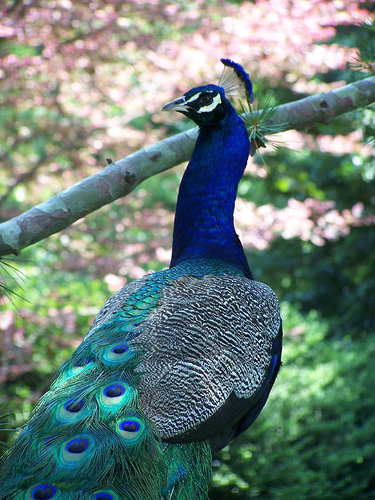
peacock_args.path = "../../tests/test_data/peacock.jpg"
data = load_and_preprocess_data(model_shape, device, peacock_args)
Image.open(peacock_args.path)
We set the mask value to zero again and predict the class of the new image.
data.set_mask_value(0)
data.target = predict_target(data, prediction_function)

print(data.target)
FOUND_CLASS: 84, FOUND_CONF: 0.51765, TARGET_CLASS: n/a, TARGET_CONFIDENCE: n/a
Next, we will run calculate_responsibility on the new image, create a MultiExplanation object, and extract explanations.
from rex_xai.multi_explanation import MultiExplanation

resp_maps, stats = calculate_responsibility(data, peacock_args, prediction_function)

multi_exp = MultiExplanation(resp_maps, prediction_function, data, peacock_args, stats)
multi_exp.extract(Strategy.MultiSpotlight)
0%| | 0/10 [00:00<?, ?it/s]
10%|█ | 1/10 [00:08<01:15, 8.42s/it]
20%|██ | 2/10 [00:13<00:53, 6.74s/it]
30%|███ | 3/10 [00:23<00:56, 8.07s/it]
40%|████ | 4/10 [00:39<01:07, 11.25s/it]
50%|█████ | 5/10 [00:47<00:50, 10.13s/it]
60%|██████ | 6/10 [00:54<00:35, 8.98s/it]
70%|███████ | 7/10 [01:02<00:26, 8.74s/it]
80%|████████ | 8/10 [01:12<00:17, 8.98s/it]
90%|█████████ | 9/10 [01:26<00:10, 10.46s/it]
100%|██████████| 10/10 [01:35<00:00, 10.14s/it]
100%|██████████| 10/10 [01:35<00:00, 9.55s/it]
Here we have used the default settings, which generate (up to) ten explanations.
The first explanation is always the explanation identified with Strategy.Global.
multi_exp.show(multi_style="separate")
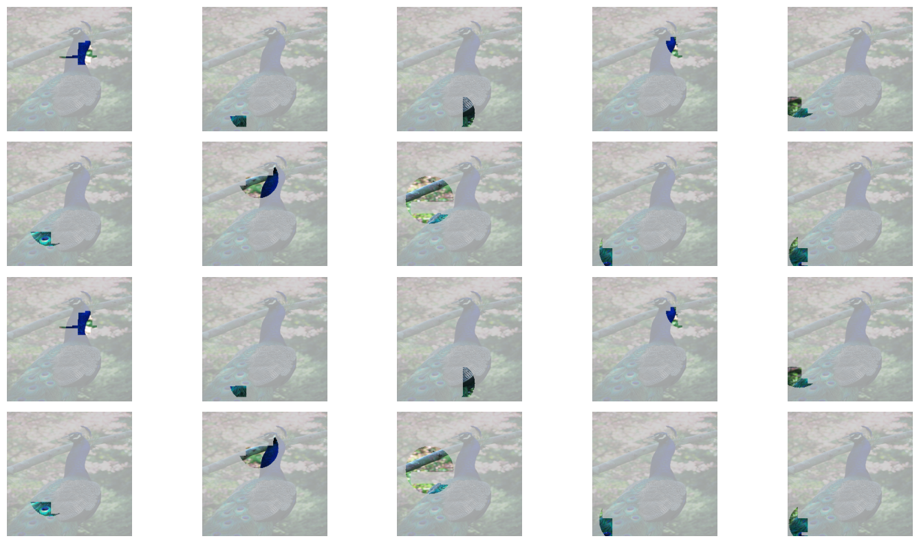
We can use the separate_by method to identify sets of explanations that do not overlap with each other (or that have an overlap less than some maximum threshold).
Here we will use an overlap of zero to find explanations that have no overlap with each other.
clauses = multi_exp.separate_by(0)
print(clauses)
[(1, 2, 3, 5, 7, 8), (1, 2, 3, 4, 5, 7), (1, 2, 3, 5, 7, 9)]
We have identified three groups of 6 explanations that have no overlap with each other. The “composite” plotting style can be used to plot these explanations in a single plot. Here we will just plot the first group.
multi_exp.show(multi_style="composite", clauses=[clauses[0]])

Saving results
We may want to run ReX on multiple input datasets and save the results for further analysis later.
We can save results from an Explanation or MultiExplanation object in a sqlite database.
We first initialise the database and then save the ladybird explanation and the multiple explanations of the peacock image.
We did not measure the time taken to calculate the responsibility landscape and extract explanations in this tutorial, so here we use zero in place of the time.
If you wish to calculate this you can use the time.time() function to calculate timestamps before and after the steps you wish to time.
Before saving the results, we should update the strategy saved in the Explanation or MultiExplanation object to ensure it matches the strategy we used, as this will be saved in the database.
from rex_xai.database import initialise_rex_db, update_database

db = initialise_rex_db("rex.db")

exp.args.strategy = Strategy.Global
update_database(db, exp, time_taken = None)

multi_exp.args.strategy = Strategy.MultiSpotlight
update_database(db, multi_exp, time_taken = None, multi=True)
ReX provides a helper function to read the results from the database into a Pandas dataframe for further analysis.
from rex_xai.database import db_to_pandas

df = db_to_pandas("rex.db")
print(df)
                     id                                path  target  \
0  -9142104089296869295   ../../tests/test_data/peacock.jpg      84
1  -6114466723269839379   ../../tests/test_data/peacock.jpg      84
2  -6077973645680009955   ../../tests/test_data/peacock.jpg      84
3  -4835238366814164447   ../../tests/test_data/peacock.jpg      84
4  -2504255480069873555   ../../tests/test_data/peacock.jpg      84
5  -1502436389336358216   ../../tests/test_data/peacock.jpg      84
6   -644286620257990681  ../../tests/test_data/ladybird.jpg     301
7   -448099728104300042   ../../tests/test_data/peacock.jpg      84
8   1727924334660682901   ../../tests/test_data/peacock.jpg      84
9   4371262226106426587   ../../tests/test_data/peacock.jpg      84
10  7548367522081723922   ../../tests/test_data/peacock.jpg      84

    confidence  time                                     responsibility  \
0     0.517648   NaN  [[34.166664, 34.166664, 39.166668, 39.166668, ...
1     0.517648   NaN  [[34.166664, 34.166664, 39.166668, 39.166668, ...
2     0.517648   NaN  [[34.166664, 34.166664, 39.166668, 39.166668, ...
3     0.517648   NaN  [[34.166664, 34.166664, 39.166668, 39.166668, ...
4     0.517648   NaN  [[34.166664, 34.166664, 39.166668, 39.166668, ...
5     0.517648   NaN  [[34.166664, 34.166664, 39.166668, 39.166668, ...
6     0.483504   NaN  [[36.0, 36.0, 36.0, 36.0, 36.0, 36.0, 36.0, 36...
7     0.517648   NaN  [[34.166664, 34.166664, 39.166668, 39.166668, ...
8     0.517648   NaN  [[34.166664, 34.166664, 39.166668, 39.166668, ...
9     0.517648   NaN  [[34.166664, 34.166664, 39.166668, 39.166668, ...
10    0.517648   NaN  [[34.166664, 34.166664, 39.166668, 39.166668, ...

   responsibility_shape  total_work  passing  failing  ... min_size  \
0            (224, 224)         980      397      583  ...       10
1            (224, 224)         980      397      583  ...       10
2            (224, 224)         980      397      583  ...       10
3            (224, 224)         980      397      583  ...       10
4            (224, 224)         980      397      583  ...       10
5            (224, 224)         980      397      583  ...       10
6            (224, 224)        1106      343      763  ...       10
7            (224, 224)         980      397      583  ...       10
8            (224, 224)         980      397      583  ...       10
9            (224, 224)         980      397      583  ...       10
10           (224, 224)         980      397      583  ...       10

            distribution  distribution_args  spatial_radius  spatial_eta  \
0   Distribution.Uniform               None            None          NaN
1   Distribution.Uniform               None            None          NaN
2   Distribution.Uniform               None            None          NaN
3   Distribution.Uniform               None            None          NaN
4   Distribution.Uniform               None            None          NaN
5   Distribution.Uniform               None            None          NaN
6   Distribution.Uniform               None            None          NaN
7   Distribution.Uniform               None            None          NaN
8   Distribution.Uniform               None            None          NaN
9   Distribution.Uniform               None            None          NaN
10  Distribution.Uniform               None            None          NaN

                     method  spotlights  spotlight_size spotlight_eta  \
0   Strategy.MultiSpotlight          10              20           0.2
1   Strategy.MultiSpotlight          10              20           0.2
2   Strategy.MultiSpotlight          10              20           0.2
3   Strategy.MultiSpotlight          10              20           0.2
4   Strategy.MultiSpotlight          10              20           0.2
5   Strategy.MultiSpotlight          10              20           0.2
6           Strategy.Global           0               0           0.0
7   Strategy.MultiSpotlight          10              20           0.2
8   Strategy.MultiSpotlight          10              20           0.2
9   Strategy.MultiSpotlight          10              20           0.2
10  Strategy.MultiSpotlight          10              20           0.2

    obj_function
0           none
1           none
2           none
3           none
4           none
5           none
6           None
7           none
8           none
9           none
10          none

[11 rows x 30 columns]
Show code cell content
import os
os.remove("rex.db")